What is this about?

As I go along my journey of picking up new concepts, I do have a desire to document some of that journey. This is my first attempt at doing so. Maybe you can learn something from this as well!

Sigmoids

Everything I learned on this subject is thanks to ritvikmath on YouTube. Here is the video I watched and will essentially be summarizing.

So, imagine we had a basketball team full of players of varying skills. After playing many, many games, we assess the overall teams performance to be $S \in (-\infty, \infty)$. Assuming we don’t know the skill rating of the other team, what would be the chance that this team wins the next game using only $S$?

Recall that the probability, $P$, by definition, must be between $0$ and $1$. Mathematically we would say $P \in (0,1)$. Now our goal becomes to do something like this:

$$S \mapsto P.$$

There is nothing too special about ”$\mapsto$.” Think of it as saying, we’re doing something to $S$ so that we get something in $P$.

Now, our goal has been defined. What step do we take to get there? A good first thought might be to define $P$ as a linear function of $S$:

$$P = cS.$$

But now we have to confine $S$ to some domain (like maybe $S \in [-100, 100]$). But the domain we choose may be arbitrary or exclusive of outliers. What if our team was GOATED and had a rating of $S = 6700$ while every team was lacking with $S = 37$ (or something like that)? Well, firstly, we should investigate this discrepancy and ensure there isn’t a crazy bias (but let’s not ruin the example).

It’s not obvious at first, but think about it. If we were given a skill rating of $S = 0$, what would this mean for our probability, $P$? Chances are, you are thinking that $P = 0.5$; that would be correct. However, this would mean there is a 50/50 chance and is equivalent to receiving no rating at all. One additional piece of info such as $S = \pm 1$ would make a significant difference.

If you are having trouble understanding this, the below example may help. (I’m trying to get better at creating examples, so bear with me!)

---

Now, think about this:

Imagine somebody came up to you with three cards ($A, B,$ and $C$). They ask you to pick a card randomly, but you are closing your eyes the entire time and some devious individual stole a card before you grab one. When you eventually select the card, you assume that there are two cards left. However, there’s only one left.

For example maybe card $A$ is left or maybe $B$ is left.
(Or maybe you’re hallucinating and you never picked up a card in the first place.)

But let’s assume you’re sane in this case (wow, I completely distracted us from the point, sorry!). The point is, you picked a card and, to an outside observer, the game is pointless because there’s obviously only one card left and thus a 100% to get only one pair. But to you, there is still a 33% chance of getting a certain pair. Having one additional piece of info drastically changed the perceived probability of a certain outcome.

---

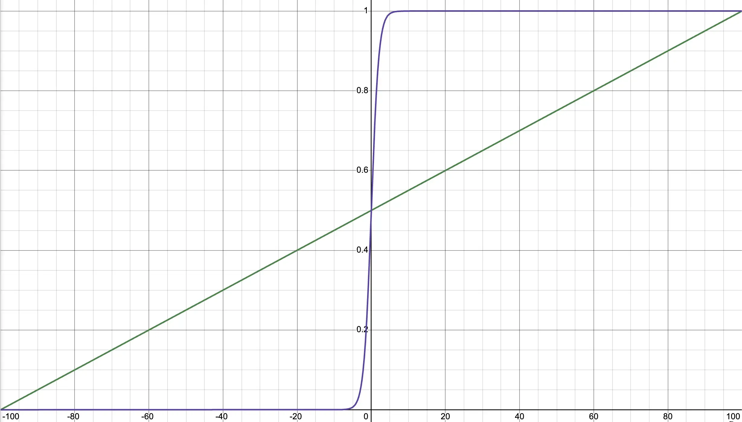
Okay, so what is the magical trick we need to do to change this? Try to picture a graph of this circumstance (if not, here’s a supplementary Desmos plot which is also shown below).

Don’t get too excited about that purple line yet, because we aren’t quite there yet. We’re at that green line, which is confined to $S \in (-100,100)$ and our probability $P \in [0, 1]$. So, we’re doing something right so far. It may be a little difficult to see, but if we make a small change to $S$ (for anyone with knowledge in calculus, we can call it $dS$) we would observe a change in $P$ (or $dP$). For our green line, that rate doesn’t change no matter where we are:

$$\frac{\text{rate of change of }P_{linear}}{\text{rate of change of }S_{linear}} = k = \frac{dP_{linear}}{dS_{linear}} \implies dP_{linear}=kdS_{linear}.$$

Now, if we want to incorporate the fact that info has a larger impact at the 50/50 point rather than elsewhere, we need the purple line. Unfortunately, I’m not sure how the equation for the purple line is derived, so I won’t show that here (maybe if I learn that later, I can come back to this).

However, the purple graph is represented by:

$$P_{adj}=\frac{1}{1+e^{-S_{adj}}} \implies \frac{dP_{adj}}{dS_{adj}} = \frac{e^{-S_{adj}}}{(1+e^{-S_{adj}})^2} = \frac{1}{1+e^{-S_{adj}}}\left(\frac{e^{-S_{adj}}}{1+e^{-S_{adj}}}\right) = P_{adj} (1-P_{adj})$$

'$_{adj}$' stands for adjusted.

Voila, we now have something that indicates a change from no information is much more significant than a change when something is obvious.

---

If that statement seems odd, think of this:

Think of a bright magenta (so insanely bright that your eyes might burn out). If you changed the hue just a little bit, it would definitely still be magenta.

Now, think of a faint magenta (or purple). If we change the hue just a bit, you may be convinced that it’s more of a blue or red-ish color (depending on whether you increased or decreased the hue).

The essence of our argument is analogous, where adding (or subtracting) info to (or from) an otherwise uninformed system is like adding (or subtracting) some hue from the faint purple: it has a more obvious difference. On the other hand, adding (or subtracting) info to (or from) a highly informed system is like adding (or subtracting) some hue from the blindingly bright magenta: it makes a minimal difference

---

Conclusion

This is about all that I have learned on this subject. I hope to gain some more knowledge (and possibly report that here) on this fascinating subject. I hope that anyone reading this has learned a little bit from me and has enjoyed reading this as much as I have enjoyed writing it.

- Cameron